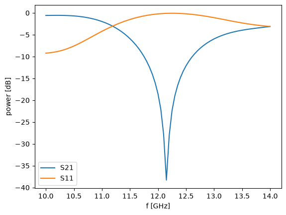
12GHz bandstop FSS: periodic metal cross array on dielectric substrate. One unit cell with periodic (Bloch) boundaries, excited by a plane wave at normal or oblique incidence theta. Compare with Tidy3D example
Setup
import os
import numpy as np
import matplotlib.pyplot as plt

import gdsfactory as gf
from gdsfactory.technology import LogicalLayer, LayerLevel, LayerStack
import luminescent as lumi

# simulation folder
path = os.path.join("runs", "FSS")

# dims [mm]
# length units are arbitrary so long as they're consistent
P = 15  # periodicity
L = 9.4  # length of cross
W = 2.0  # width of cross stub
h_sub = 2.2  # substrate thickness
h_metal = 0.1  # metal thickness

# frequencies [GHz]
# spectrum computed from single FDTD run. more frequencies slightly increases runtime
frequency = 12
bandwidth = 4
nfs = 81
frequencies = np.linspace(frequency - bandwidth / 2, frequency + bandwidth / 2, nfs)

c0 = 300  # speed of light [mm GHz]

# incidence angle [degrees] from z in xz plane. E along y (TE)
theta = 0

def setup(path, frequency, frequencies, P, L, W, h_sub, h_metal, theta):
    # simulation parameters
    nres = 16
    dx = W / 8  # desired resolution near metal
    stop_decay = 1e-3
    PML_decay = 0.001  # x y z
    courant = 0.9
    subpixel_smoothing = 1
    shot_every = 2.5  # movie [periods]
    views = [lumi.view("Ey", z=h_metal / 2)]

    # one unit cell, periodic in x y. Bloch wavevector sets incidence angle (exact at center frequency)
    boundaries = ["periodic", "periodic", "PML"]
    k_bloch = lumi.bloch_wavevector(theta, 0, dim=3, f=frequency, c0=c0)

    # margins
    # air gap keeps evanescent resonant field from coupling to PML
    gap = 30.0
    source_offset = 2.0

    # vertical dims
    z_o1 = h_metal + gap
    z_o2 = -h_sub - gap
    zmin = z_o2
    zmax = z_o1 + source_offset

    # materials
    # refine mesh in substrate and metal: n sets mesh density relative to vacuum
    n = (c0 / frequency / nres) / dx
    materials = {
        "air": lumi.material(1),
        "sub": lumi.material(epsilon=2.5),
        "PEC": lumi.PEC_material(n),
    }
    background = "air"

    # layers
    METAL = 1, 0
    SUB = 2, 0
    layer_stack = LayerStack(
        layers={
            "metal": LayerLevel(
                layer=LogicalLayer(layer=METAL),
                thickness=h_metal,
                zmin=0,
                material="PEC",
                mesh_order=1,
            ),
            "sub": LayerLevel(
                layer=LogicalLayer(layer=SUB),
                thickness=h_sub,
                zmin=-h_sub,
                material="sub",
                mesh_order=2,
            ),
        }
    )

    # make component in gdsfactory. alternatively can import .gds into gdsfactory
    # cross unit cell centered at origin
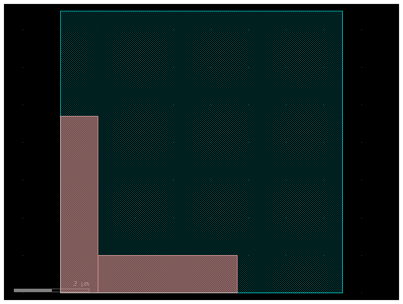
    c = gf.Component()
    c.add_polygon([(-W / 2, -L / 2), (W / 2, -L / 2), (W / 2, L / 2), (-W / 2, L / 2)], layer=METAL)
    c.add_polygon([(-L / 2, -W / 2), (L / 2, -W / 2), (L / 2, W / 2), (-L / 2, W / 2)], layer=METAL)
    c.add_polygon([(-P / 2, -P / 2), (P / 2, -P / 2), (P / 2, P / 2), (-P / 2, P / 2)], layer=SUB)
    c.plot()

    bbox = c.bbox_np().tolist()
    bbox[0].append(zmin)
    bbox[1].append(zmax)

    # sources, monitors
    # plane wave on face frame spanning the cell. E along y, H along x
    # wave admittance in air: Hx/Ey = cos(theta) in magnitude (sign fixed automatically)
    frames = [lumi.face("plane_wave", modes=[[{"Ey": 1, "Hx": -np.cos(np.deg2rad(theta))}]])]

    # dim: outward normal axis. source injects into cell, monitors record in (-) and out (+) waves
    sources = [
        lumi.source(
            "o1", z_o1 + source_offset, dim=3,
            frame="plane_wave",
            f=frequency,
            bandwidth=max(max(frequencies) - min(frequencies), frequency / 4),
        )
    ]

    monitors = [
        lumi.monitor("o1", z_o1, dim=3, frame="plane_wave"),
        lumi.monitor("o2", z_o2, dim=-3, frame="plane_wave"),
    ]

    # writes .obj mesh files from gdsfactory component
    lumi.mesh(path, c, layer_stack, materials, zmin, zmax)

    # writes setup file
    lumi.setup(
        path=path,
        f=frequency,
        fs=frequencies,
        c0=c0,
        materials=materials,
        background=background,
        boundaries=boundaries,
        k_bloch=k_bloch,
        bbox=bbox,
        #
        frames=frames,
        sources=sources,
        monitors=monitors,
        #
        nres=nres,
        courant=courant,
        PML_decay=PML_decay,
        subpixel_smoothing=subpixel_smoothing,
        #
        views=views,
        shot_every=shot_every,
        stop_decay=stop_decay,
        device="gpu",
    )


setup(path, frequency, frequencies, P, L, W, h_sub, h_metal, theta)
lumi backend: None
using simulation folder runs/FSS
Solve
lumi.solve(path)========================================
backend using simulation folder runs/FSS
========================================
setting up simulation...
processing geometry bodies...
generating voxels...
subpixel smoothing: 1.629317 seconds (9.74 M allocations: 431.472 MiB, 2.56% gc time, 224.68% compilation time)
making sources o1 ...
making monitors o1 o2 ...
========================================
run: runs/FSS
processor: CPU
cpu threads: 16
nres: 16.0
courant: 0.9
subpixel_smoothing: 1
boundaries: [:PEC :PEC; :PMC :PMC; :PML :PML]
sources
o1: 0, 0, 32.1
monitors
o1: 0, 0, 30.1
o2: 0, 0, -32.2
original size: (24, 24, 57)
padded size: (24, 24, 91)
cell count: 52,416
step size: 321.0 steps/period
source duration: 3 periods
max time: 100 periods
max steps: 32,100
max load: 1,682,553,600 cell-steps
energy decay threshold: 0.001
========================================
running simulation...
accumulating dft field...
period 2.5, 4.33 seconds/period
period 5.0, decay: 0.325, 0.121 seconds/period
period 7.5, decay: 0.035, 0.091 seconds/period
period 10.01, decay: 0.002, 0.094 seconds/period
period 10.77 stop on energy decay
simulation completed.
Movie
lumi.movie(path)Video generated successfully at runs/FSS/Ex_0_0_0.05.webp!
Loading...
Results
sol = lumi.load(path)
o1 = sol["monitors"]["o1"]
o2 = sol["monitors"]["o2"]

# + denotes outgoing mode (wrt port monitor outward normal), - incoming
S21 = o2["modes"][0]["+"] / o1["modes"][0]["-"]
S11 = o1["modes"][0]["+"] / o1["modes"][0]["-"]

plt.figure()
plt.plot(frequencies, 10 * np.log10(np.abs(S21)**2), label="S21")
plt.plot(frequencies, 10 * np.log10(np.abs(S11)**2), label="S11")
plt.xlabel("f [GHz]")
plt.ylabel("power [dB]")
plt.legend()
plt.show()
loading solution from runs/FSS
may take a minute if simulation folder is remotely mounted